The Belfry

In an earlier post, I described an “inverse” RIAA equalization circuit. This mimics the recording curve used when cutting a modern record. In that post, along with a brief description of phono equalization, I gave the equations for calculating the resistor and capacitor filter values for the RIAA equalization curve and for that specific circuit. Here, let’s take a look at the general equations used for these curves.

The following shows the basic equalization circuits and the corresponding equations for both the playback and recording curves.

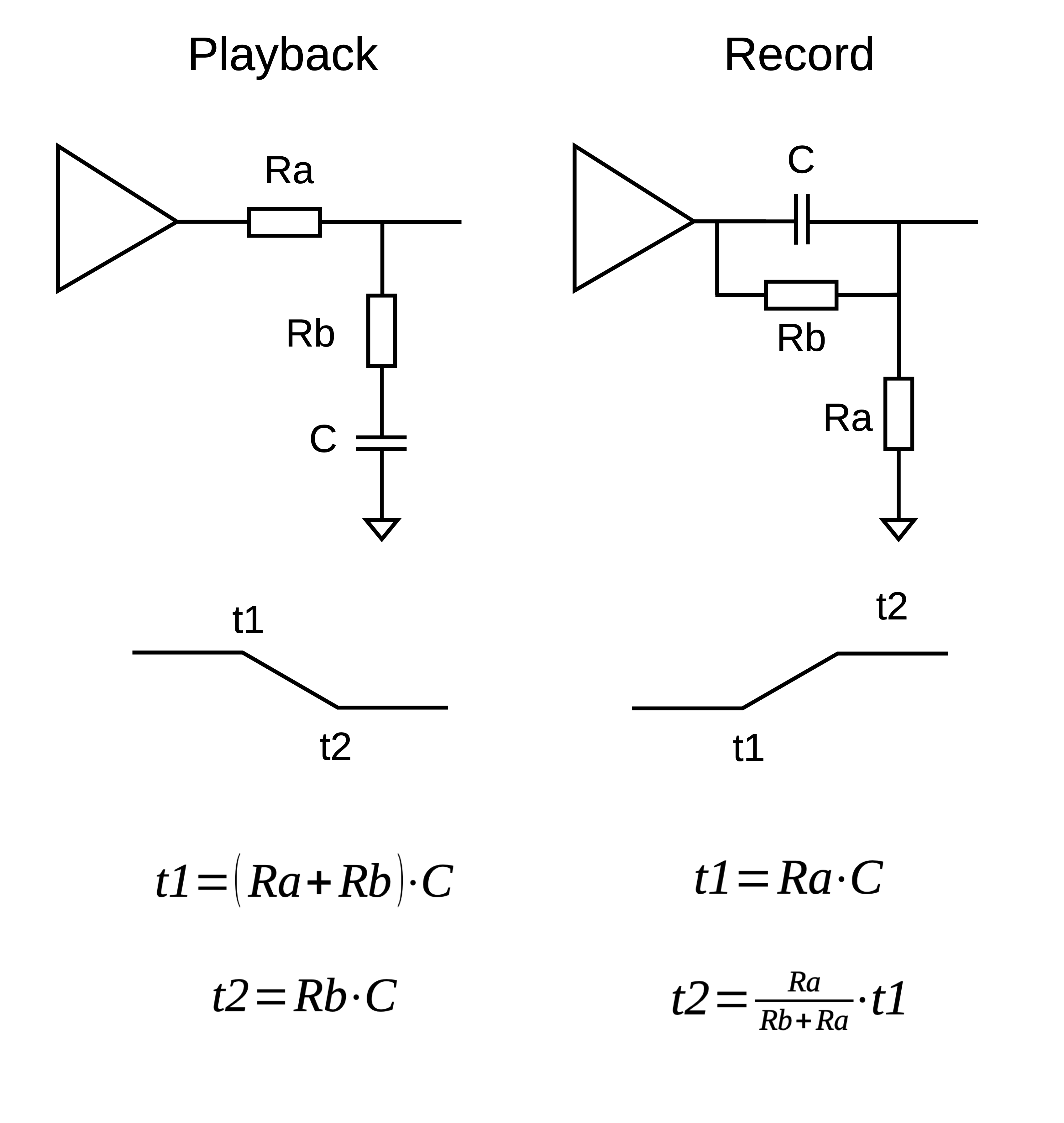
This is meant for use in a two-stage active equalization circuit. Shown are the equations for an individual stage. Both stages use the same circuit with the two stages in series. One for the lower frequencies (20Hz-1kHz), the second for the higher frequencies (1kHz-20kHz). (I’m keeping this to the audio range.) Each stage has filter nodes or knees at two frequencies. These nodes, labeled t1 and t2 in the chart, are specified by their time-constant. You can convert between the time-constant and frequency with these equations.

For RIAA equalization (both playback and record), the first stage uses the time-constants 3180µs (50Hz) for t1 and 318µs (500Hz) for t2. The second uses 75s (2122Hz) for t1 and 3.18µs (50kHz) for t2.

The RIAA standard

The RIAA curve only defines three nodes at 50Hz, 500Hz, and 2122Hz. Additional nodes have been proposed as well. One at 20Hz (7950µs), the IEC amendment, is intended to help minimize turntable rumble or improve low-frequency accuracy. That is not included here. The 50kHz node is called the Neumann constant, named for a manufacturer of cutting lathes. This is to minimize ultrasound artifacts going to the cutting head. There is some controversy regarding this extra nodes and any investigation will take you down quite a rabbit-hole. One side-effect of the Neumann constant is its influence on lower frequencies, shifting the curve by ~1dB at 20kHz. It can be that the Neumann pole was used for some recordings and is included here. I don’t consider ±1dB at the frequency extremes to be an issue. These equations include it.

These equations solve for the time-constants. But we already know the constants and want values for the resistors Ra and Rb and the capacitor C. Using algebra, you can re-arrange the equations to solve for these values. The only one that gets a bit tricky is calculating the t2 values for the record curve. If you have a calculator with an equation solver (I used an HP-48GX), this can be handy. Another option is WolframAlpha. For example, to calculate Rb knowing Ra and C, in the input field type:

solve t2=(R1/(R2+R1))*t1 for R2

Hit Enter and it returns:

(I had to substitute R1 for Ra and R2 for Rb otherwise WolframAlpha got confused.)

Of course, you can just plug in the known values in the input field to get the answer.

Final observations

As I mentioned earlier, these equations are for a two-stage active filter. Single-stage and passive filters can also be built and many suggested circuits can be found in books and online.

These are simplified equations derived from much more complex formulae. I am not an engineer and my math is not up to calculating from first principles. The equations here are well known and found in many resources. “On the shoulders of giants…” This documents my attempt to wrap my head around how to use them.

In the process, my way of thinking about what is going on landed on the idea that each stage is really just a low-pass filter (high-pass for the record curve) with the node at t1. The curve then has a kind of leveling-off or shelf defined by node t2.

In any case, the equations presented here work and made the task of defining a proper filter much easier than many of the other articles I’ve seen. Finally, I’d like to say that though these equations will get accurate values for the filter components, my experience is that close does count. I’ve been happy with errors of even many tenths of a decibel which simplifies things a lot. But you do you.