The Belfry

The problem I wanted to address is the difficulty in testing a HiFi phono-stage using a bench audio frequency generator. The signal from the cartridge is a few millivolts for a moving-magnet type down to a few hundred microvolts for a moving coil cartridge. Most hobby-level frequency generators just won’t deliver a clean signal at these levels. And you have to control that level for different frequencies to keep the output of the phono-stage constant. The solution is a circuit that takes a constant level from the audio source and delivers the appropriate low-level equalized signal to the device under test.

There are numerous posts on the net that describe equalization and circuits to do both playback and recording equalization. You may already have a good idea how equalization works and seen other’s posts. If you’re just interested in the circuit, you can skip a lot of what follows. If you’re approaching this as I first did, my aim here is to distill what I learned to provide the basic information needed to understand and solve the problem.

The circuit described here is pretty basic textbook stuff. One source that was of particular help to me in defining the circuit is at https://next-tube.com/articles/eriaa/eRIAA_en.inc

Phono equalization—a brief overview

The first step in record manufacture is to make a master impression of the record. This is done by cutting the grooves into a disc of lacquer. Think of the thing that does the cutting, the cutting head, as something like the cartridge in your record player but working in reverse. And the stylus as a little chisel. Instead of generating a signal, an audio signal is sent to this cutting head which forces the chisel tip to wiggle in step with the signal.

However, the audio from the master tape or other source is altered before being sent to the cutting head. The low frequencies are reduced and the high frequencies are boosted. This is done so that when the record is played, the stylus is not driven too hard by bass content and, the extra treble level can help to reduce noise.

But for this to work, when the record is played the phono-stage has to reverse that alteration. That is, it has to boost the bass and reduce the treble (which also reduces the inherent hiss). This is equalization. In the early days of record production there were many equalization curves in use. Eventually a curve defined by the Recording Industry Association of America became the standard. It’s called, logically enough, RIAA equalization. By the 1950’s nearly all record and preamp manufacturers used it. (There were some exceptions. For example, in Germany and a few other European countries, many record companies used a slightly different curve named TELDEC/DIN. This doesn’t apply here but will in some later posts.)

What does that look like?

To visualize what’s going on, here’s a graph of the RIAA equalization recording- or inverse-curve. (The playback curve, the one in the pre-amp, is the same but flipped upside down. If the record is made using the curve shown, the pre-amp will flatten the signal.)

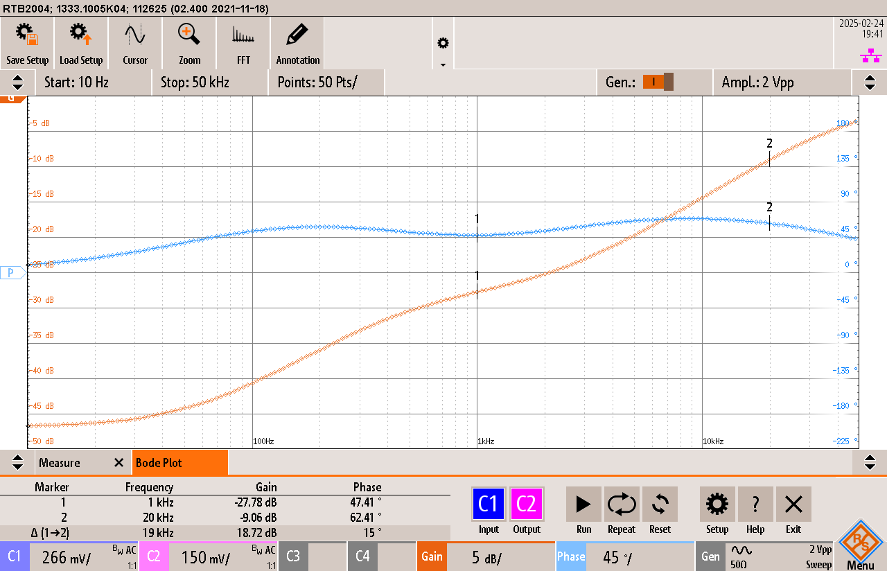
The RIAA equalization curve is in orange. (The blue curve is the phase shift. Not important here.) This is a Bode plot that shows the difference in the signal level between the input and output for a range of frequencies. This was generated using the circuit described here and matches the true curve quite closely. The X-axis is the frequency, The frequencies plotted are from 10Hz to 50kHz. The Y-axis is the level difference in decibels or dB. This is a logarithmic measure. Twenty decibels corresponds to a factor of ten. That is, 20dB is a ten times difference, 40 dB another ten or a hundred times and so on.

We need attenuation, too

In addition to equalization, the circuit also needs to attenuate, or reduce, the signal from the comparatively high output level of the test signal source to the low level expected by the phono-stage input. You can see that the measured attenuation factor is -27.78dB or about 4.1% of the input (marker 1 on the graph and noted near the bottom-left of the image). This is at 1000Hz, the reference or middle frequency of the curve. This translates to an output level of about 30mV RMS for an input of 707mV RMS or 2V peak-to-peak.

Decibel vs. voltage difference equations

Here are the equations used for going between decibels and voltage difference.

voltage difference to decibels:

decibels to voltage difference:

Where Lvl is the decibel value dB, Vref is the reference or input value in volts, and V is the output value in volts.

A great resource for these and many more electronics-related formulae as well as online calculators is at https://sengpielaudio.com/calculator-db.htm

The curve in more detail

Ideally, at 20Hz, the curve is 20dB lower than the reference or -47.78dB. The graph shows about -46.5dB. This is within the tolerance expected from the resistor/capacitor values I used and is acceptable for my use. At 20kHz (marker 2) the attenuation should be 20dB above the reference or -17.78dB. The measured value is -18.72. Close as well but there is another reason for that ~1dB difference here.

Filter nodes

The curve is produced using filters—most often with a resistor/capacitor network. These are chosen for the specific frequencies where the curve needs to bend. I’m calling them nodes here. This is the inverse equalization plot again, this time with the nodes marked.

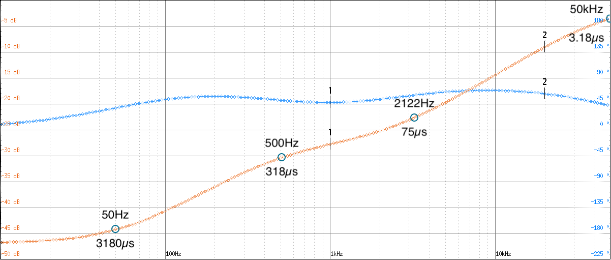
The RIAA curve defines three nodes at 50Hz, 500Hz, and 2122Hz. These are actually specified by their time-constants which are 3180µs, 318µs, and 75µs, respectively. I’ll refer to those from here on.

Frequency vs. time-constant equations

You can convert between the frequency and time-constant using the following equations.

Where f is the frequency in Hz and τ (tau) is the time-constant in seconds.

Additional nodes have been used as well. One at 7950µs (20Hz), the IEC amendment, is intended to help minimize turntable rumble or improve low-frequency accuracy. That is not included here. Another is at 3.18µs (50kHz) and called the Neumann constant, named for a manufacturer of cutting lathes. This is to minimize ultrasound artifacts going to the cutting head. There is some controversy regarding these extra nodes and any investigation will take you down quite a rabbit-hole. One side-effect of the Neumann constant is its influence on lower frequencies, shifting the curve by ~1dB at 20kHz. It can be that the Neumann pole was used for some recordings and is included here. I don’t consider ±1dB at the frequency extremes to be an issue. And the equations I used included it (see the article I referenced way back at the beginning).

The circuit

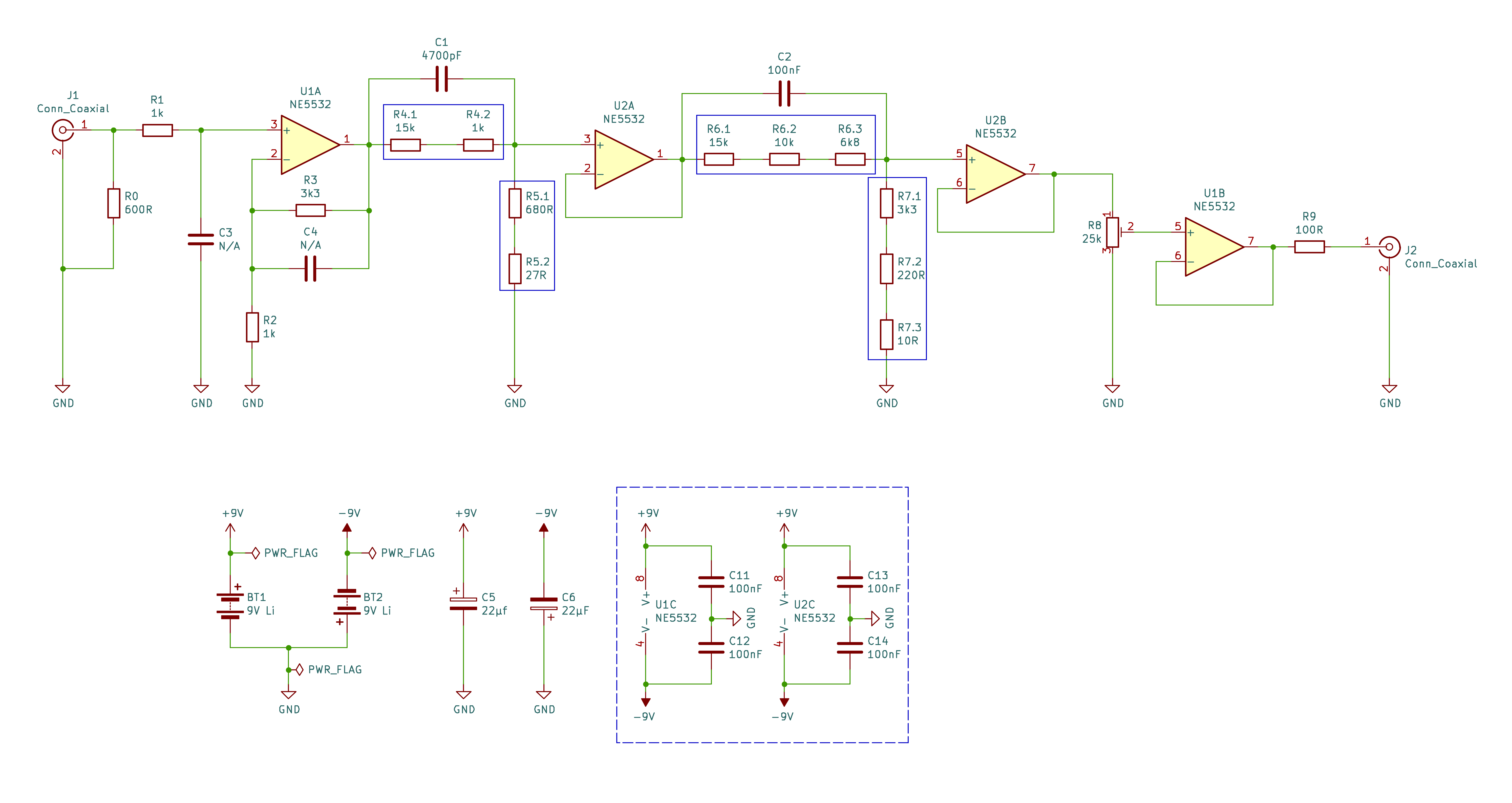
Finally, we come to the circuit I used. As I mentioned, there are many circuits out there, some passive (no active components), others are active using tubes, transistors, or op-amps. This is an active circuit using common op-amps. Here is the schematic.

I think the circuit is pretty straight-forward so I won’t go into detail about it. But here are a few points.

• The first stage, op-amp U1A and the filter components C1, R4, R5 set the 75µs and 3.18µs nodes. U2A and C2, R6, R7 set the 3180µs and 318µs nodes.
• For the filter components C1, R4, R5 and C2, R6, R7 you can use the values shown or change them based components you have on-hand. I’ll discuss the equations to do that below.
• The resistors R2, R3 set the gain of the first stage. Here the gain is 4.3. You may want to experiment with the gain depending on input level. This is about 2V PP, 707mV RMS for 30mV RMS out for my use. If the gain is too high the op-amp may clip.
• Capacitors C3, C4 are not used. C3 would filter ultra-sonics if that’s a problem. C4 may be needed if the op-amp is unstable. Low values, a few pF, would be fine.
• Since I used battery power, the smoothing capacitors C5 and C6 are probably not needed. They’re there because I initially intended to use USB power with a 5V to ±15V converter module. However, this proved to be too noisy.

Adjusting the filter component values

My choices for the node filter component values were driven by what I had on-hand. Yours may be too. Here are the equations needed to calculate the values and a description how to apply them.

Since capacitor values are usually more limited than resistor values in your parts bins, these equations start with selecting the capacitor values. The equations will then give you the two resistor values for each stage, the first below 1000Hz and the second above 1000Hz. Note that in the equations, the capacitor values are in Farads and the node values are in seconds. The component identifiers are the same as on the schematic.

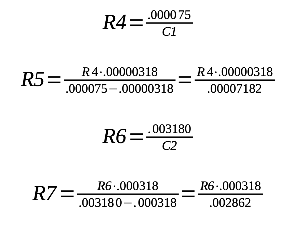
Using the capacitor values in the schematic, here is an example of the calculations.

• For the 75µs node, C1=4700pF (.000000004700F)so R4=15957Ω
• For the 3.18µs node, use the R4 value to get R5=706.55Ω
• For the 3180µs node, C2=100nF (.000000100F) so R6=31000Ω
• For the 318µs node, use the R6 value to get R7=3533Ω

I chose a combination of resistors in series to get close to the calculated values. It’s also a good idea to measure the capacitor value with an accurate LCR meter (not the capacitor function on a multimeter) and use that.

The general equations

The equations above have been simplified to be specific to this application. They are derived from more general equations as presented in numerous other resources and are based on my limited understanding of the math and engineering involved. But they do provide the correct numbers!

In this post I describe how I got to these simplified equations.

Construction

Of course you can use pretty much whatever construction that works for you. Following is a very brief view of what I did.

The device is housed in an old pipe tobacco tin.

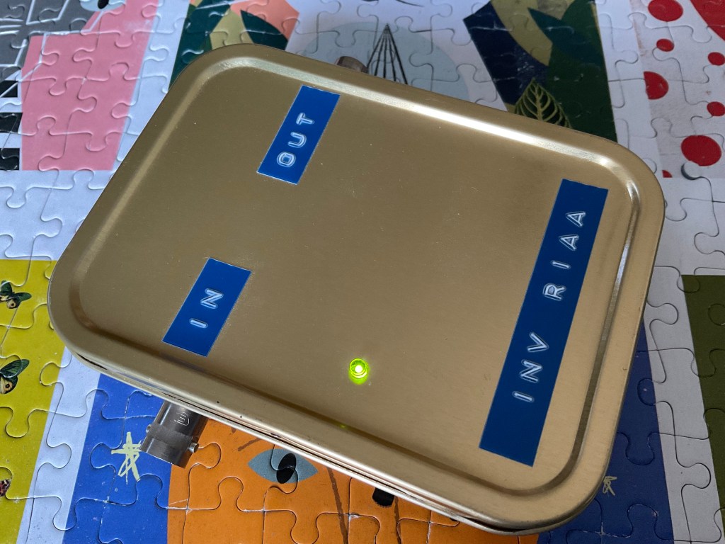
Here’s the inside.

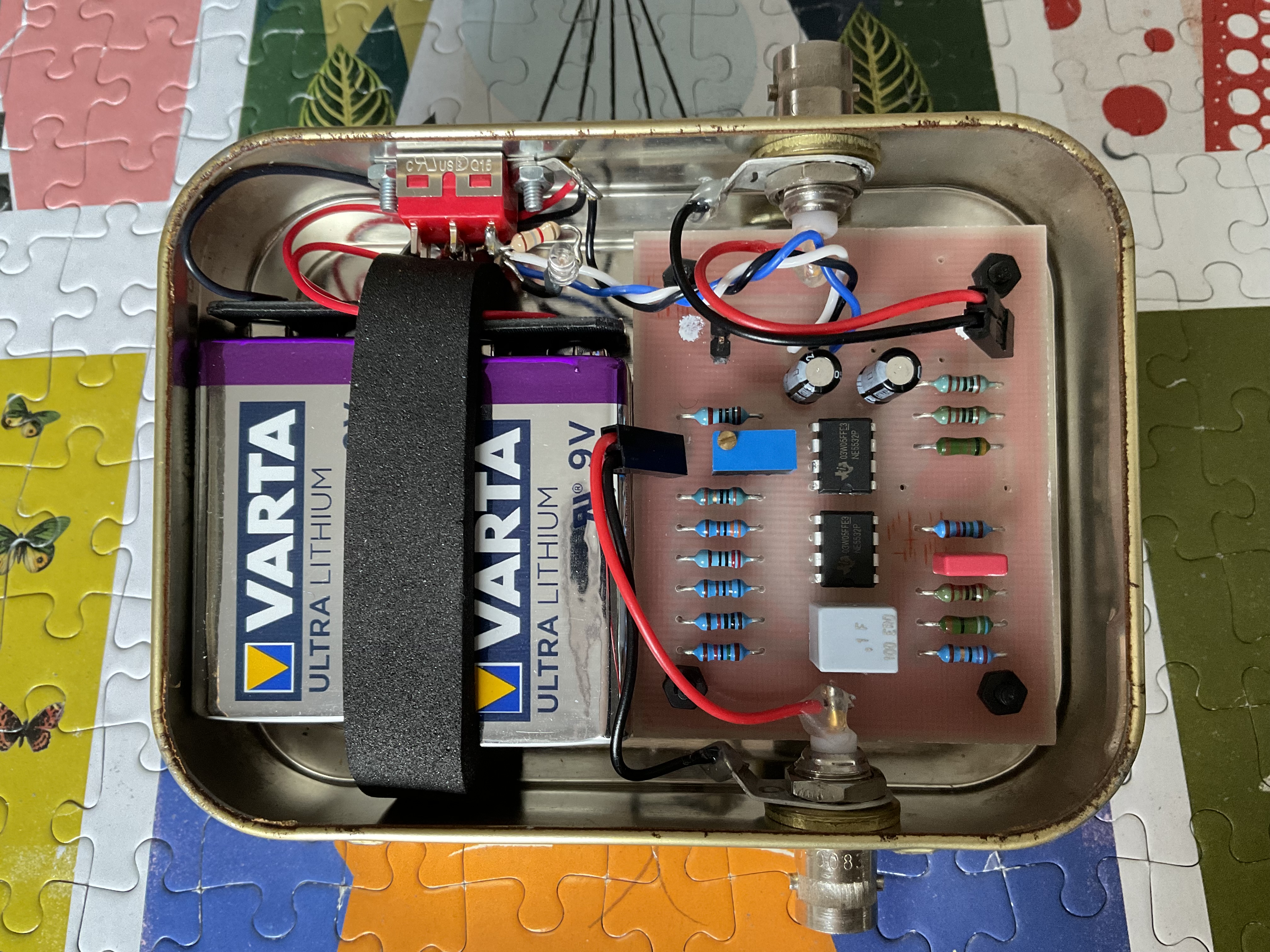
And the PC board. I made it using a cheap milling machine.

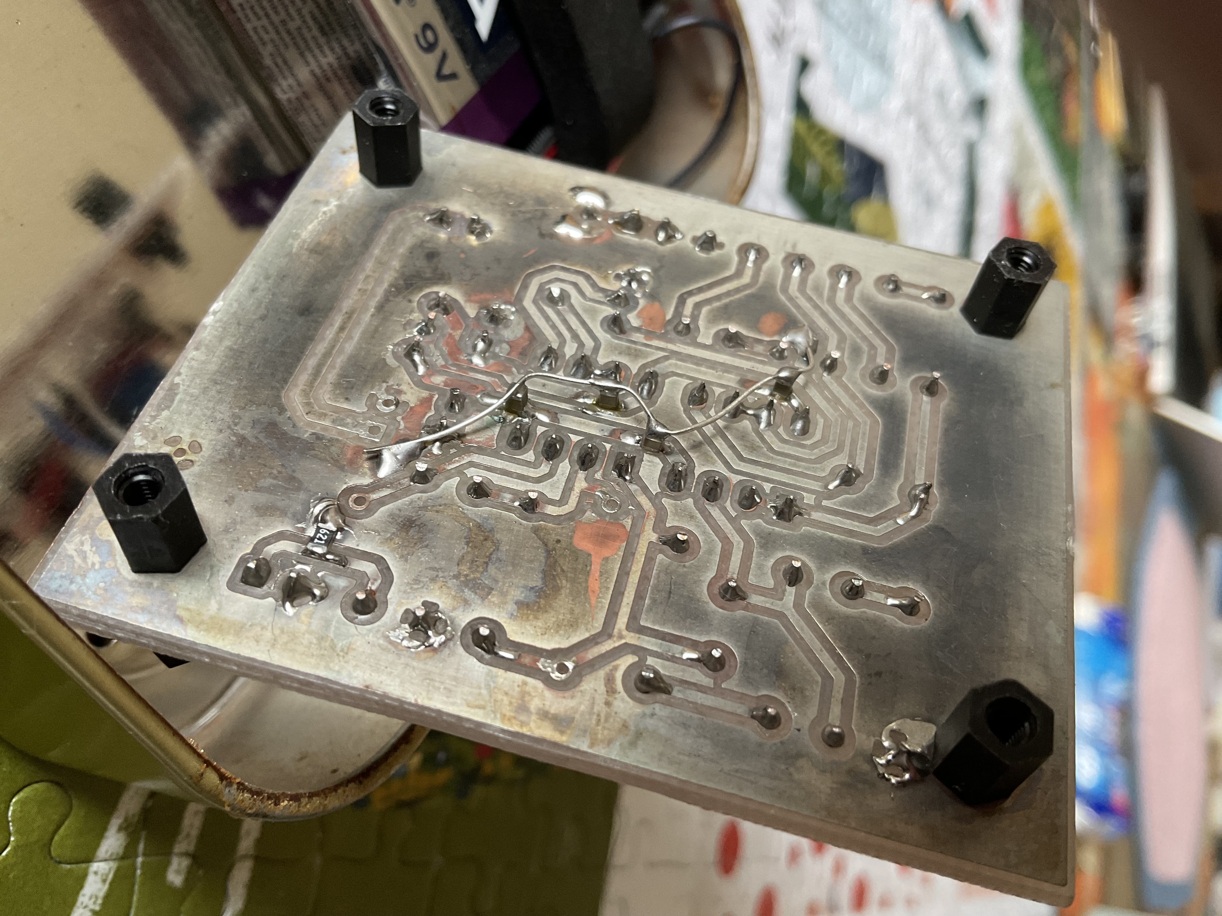
On the board underside you can see that the IC bypass capacitors C11-14 and the input impedance resistor R0 are bodged using SMD parts.

I used KiCad. Here’s the copper and parts layout. It’s pretty basic as all I needed was the copper layer and a drilling file.

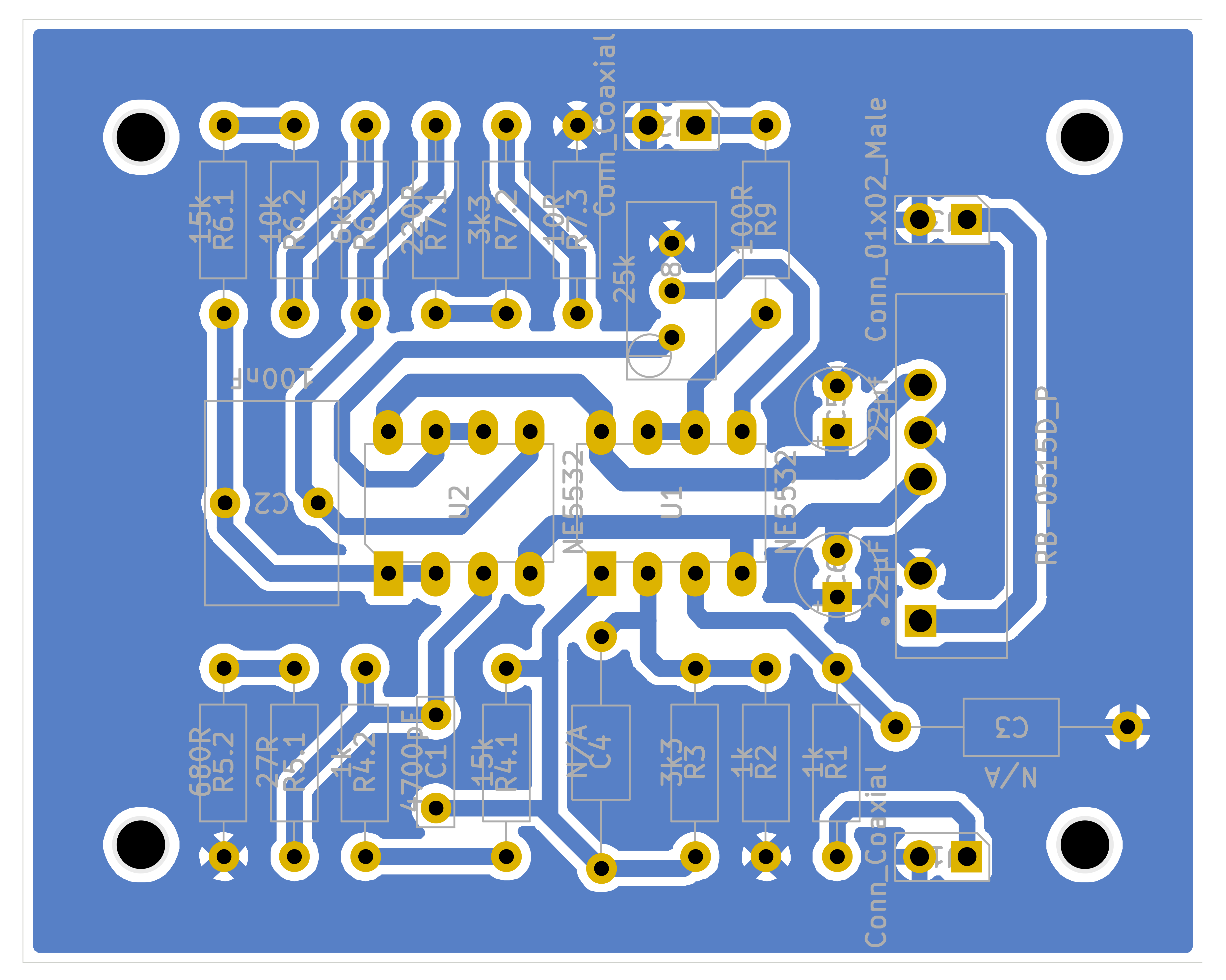
If they can be of use, here are the KiCad files.

Conclusion

It was quite a journey to get here. I saw the need for such a piece of test equipment when I planned the construction of a vacuum tube phono preamp. (Stay tuned. Future posts will document my development of a complete mono LP playback system that could have, feasibly, been built circa 1960.) Many net searches later and the result you see here emerged. As I said at the beginning, if you need such a device, this is my attempt to make your journey just a bit easier, highlighting the basic information to get there.

Thank you for reading this far. Was it too light? Not detailed enough? Are there glaring errors? Probably yes to the later. I would really like to hear your comments.